Reinforcement Learning for Intersection Traversal
Introduction
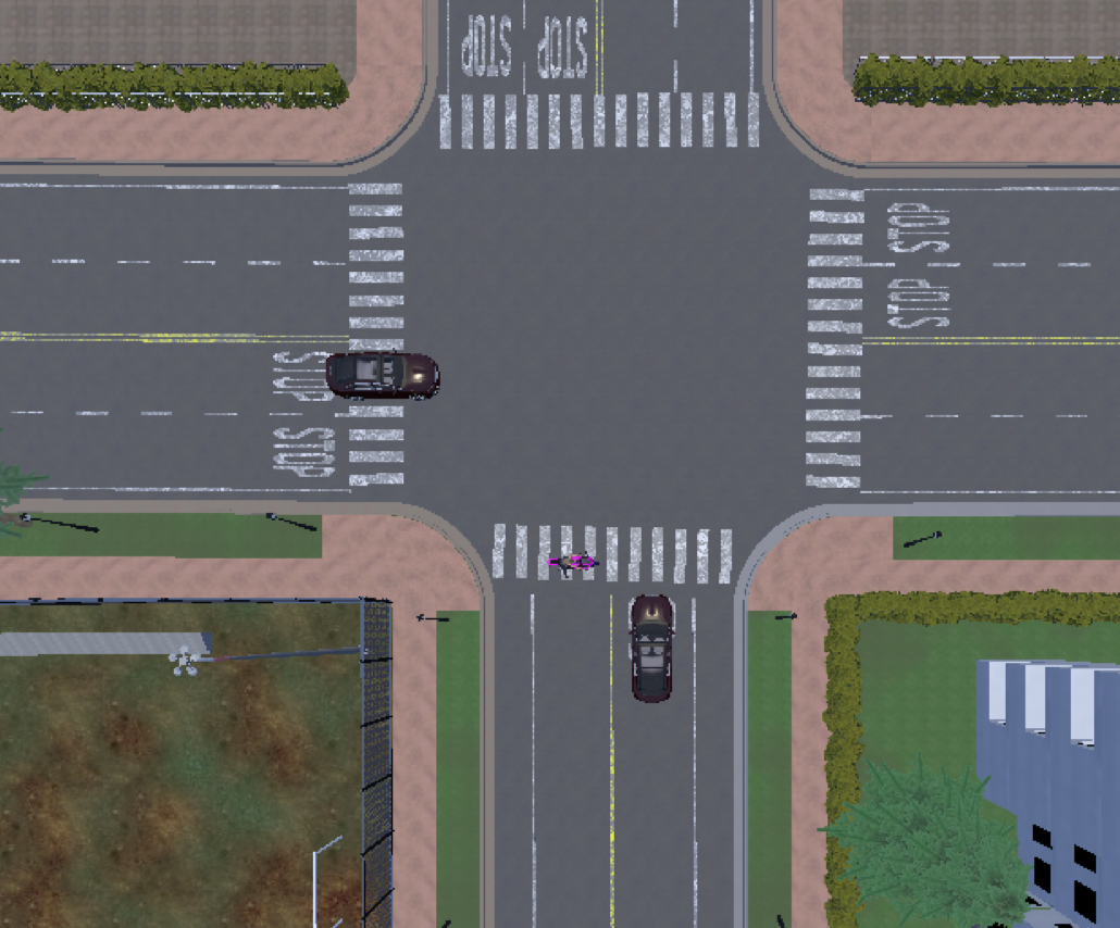
In this report we examine the problem of intersection crossing for autonomous driving. We consider the case of an unprotected intersection where non-ego agents do not yield to the ego vehicle as it makes a left turn. We assume that the state of the ego and the states of non-ego actors are fully observable. See Fig. 6 in Appendix Background for details.
The task is implemented in the Carla simulator for automated driving, and is tackled using a combination of empirical evaluations and algorithm developments. We begin with evaluating a suite of model free algorithms’ ability to solve the task: SAC, PPO, and TD3. Then, curriculum learning and hierarchical planning algorithms are applied to improve the learning performance and ensure passenger comfort, respectively.
Empirical Evaluation
In this section we adapt existing model free RL techniques to the proposed task. Specifically, three model free algorithms are chosen and adapted to the task: SAC, PPO, and TD3.
MDP Formulation
To apply the model free algorithms, the task is cast as a Markov Decision Process (MDP) defined as follows:
State: The state provided to the agent contains the velocity, acceleration, yaw angle, yaw rate, and lateral deviation from lane center of the ego vehicle. The state also contains the yaw angle of the lane at an interval of 5, 10, and 15 meters in front of the ego, which is necessary to track the lane center. Finally, in the simplest setting with a single target (non-ego) vehicle, the state also contains the relative lateral and longitudinal distance between the target and ego vehicles, as well as the target’s velocity. In later mentioned experiments where the number of non-ego actors is expanded, the state of the additional actors is handled in a similar fashion.
Reward: The reward function required a heavy amount of shaping to yield good learning performance. The desired driving behavior is to proceed to the end of the route (completing the left turn) as efficiently as possible while remaining safe (in lane and no collisions). We found that a progress-along-route reward did not lead to efficient completion because the agent was encouraged to take many steps to gather more reward. Instead, a negative reward for distance-to-goal did encourage efficient route completion. Furthermore, a positive reward is given for high speeds that remain under the speed limit of 12m/s, while negative rewards are given for exceeding the speed limit. A negative reward is given proportional to lateral deviation from the lane center. Finally, in the terminal case of route completion, a large positive reward is given, but in the terminal case of a collision a large negative reward is given. The final reward function is:
\[R(s,a) = c_1*v_{eff} + c_2*lat_{dev} + c_3*dist_{goal} + term \tag{1}\]where \(v_{eff}\) is the difference between the speed limit and the ego’s speed (negative when over the speed limit). Furthermore, \(term\) is 100 in the case of route completion, -10 in the case of collision, and 0 otherwise. \(c_1, c_2, c_3\) are weighting constants that were tuned experimentally to be \(1.0\), \(0.1\), and \(3.5\) respectively.
Action Space: In the original task formulation the agent controls the low level (throttle and steering) states directly. It does so by choosing a delta action that is added to the current throttle and steering states. In Section [4] when we talk about introducing a low-level controller between the actor and the environment, the action space of the agent will change to higher level commands, specifically reference velocity and yaw angle.
Implementation
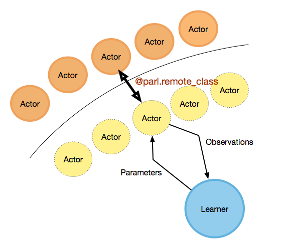
The framework in which the algorithms were implemented is PARL. PARL was chosen because it allows for distributed training, see Fig. 6 in Appendix Background, which is necessary to collect a large volume of experiences on the relatively slow Carla simulator. Additionally, PARL offers existing implementations of popular model free algorithms on the Mujoco task set, which we were able to adapt to the Carla based environment we propose.
One implementation detail that we found effective was to schedule the entropy bonus \(\alpha\) used in SAC based on the success rate of the task. Specifically, we used
\[\alpha = clip(1 - \lambda, 0.1, 0.3) \tag{2}\]where \(\lambda\) is the success rate over the past 10 evaluation episodes.
Results and Discussion
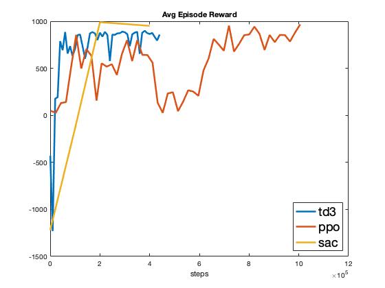
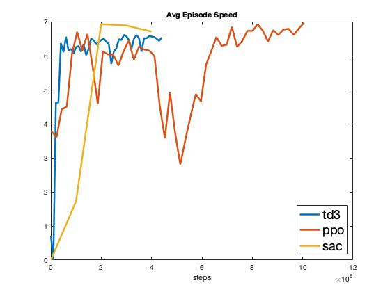
A selection of results from the model free algorithm experiments can be found in Fig. 1. As seen in Fig. 1, SAC outperforms both TD3 and PPO in terms of maximizing cumulative reward. However, TD3 is able to learn with very few samples, on the order of 10k, whereas SAC requires an order of magnitude more samples and does not converge until 200k samples. This agrees with the theoretical groundings presented in [@fujimoto2018addressing] that a double-critic architecture improves the learning performance by reducing the overestimation bias. However, SAC does eventually achieve a higher reward compared to TD3, this can be attributed to the entropy bonus in SAC allowing it to discover a better policy via exploration [@haarnoja2018soft]. PPO takes the largest number of policy updates to converge, which can be attributed to its proximal optimization nature discussed in [@schulman2017proximal].
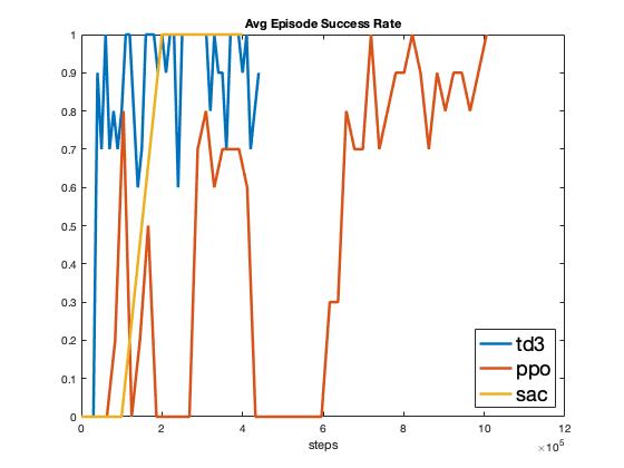
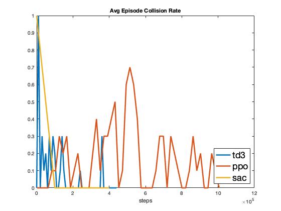
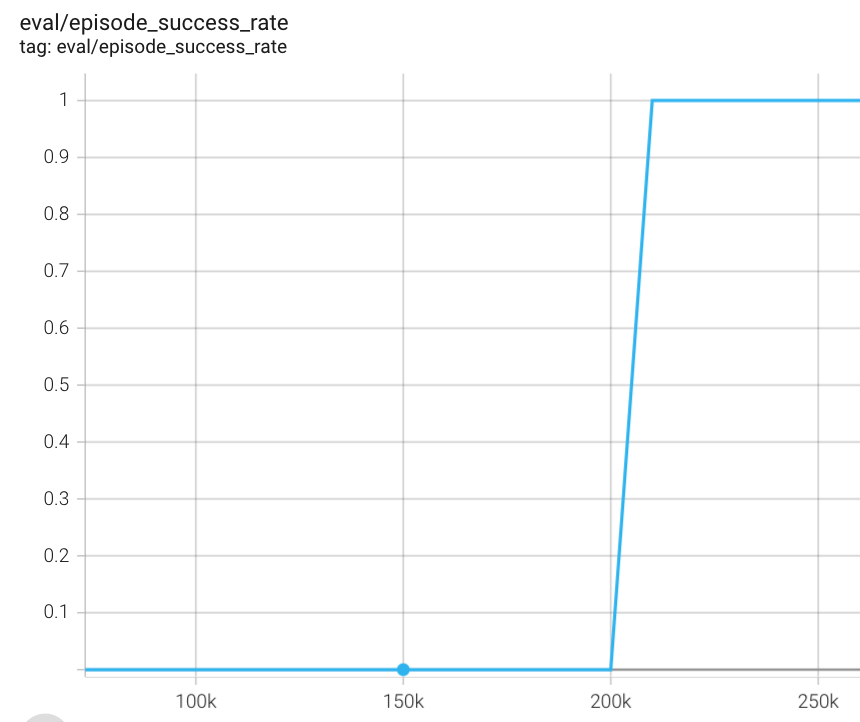
As seen in Fig. 1, SAC also achieves a consistently perfect success rate upon learning convergence, whereas TD3 and PPO also eventually achieve a perfect success rate but never consistently. SAC’s consistency can be attributed to the \(\alpha\) scheduling term introduced in Eq. (2). As seen in Fig. 1, the collision rate follows the same general pattern, with only SAC achieving a consistently collision free policy. Lastly, it is interesting that all three policies converge to the same average speed of 6.5 m/s (Fig. 1), indicating that 6.5 m/s is the most efficient speed to complete the route while avoiding the target vehicle.
Algorithm Design I: Curriculum Learning
We were unsatisfied with the inconsistent performance of TD3 and the large magnitude of experiences required by SAC to achieve perfect consistent success. Thus we moved forward with investigating the usefulness of curriculum learning (CL) applied to our task.
Background
CL was proposed in [@bengio2009curriculum] as a way to accelerate learning by first training the system on simple tasks and before progressively increasing the difficulty of the tasks given to the learning agent. Recently, CL as been applied to learning high-speed autonomous overtaking [@song2021autonomous]. Furthermore, manually designed curriculum has also showed learning benefits in terms of training time reduction and faster convergence in urban driving settings at unsignalized intersections. For instance, in [@qiao2018automatically], a CL based RL scheme was proposed for crossing a four-way unsignalized intersection autonomously. The proposed algorithm was designed to automatically generate curriculum in order to learn the crossing policy with fewer training iterations. However, in that work only simple one-dimensional crossing behavior is learned, while other more complex scenarios. i.e. two-dimensional left-turn was not investigated.
Handcrafted Curriculum
We began our investigation using a manually designed curriculum. The agent is first tasked to follow the lane center without any non-ego actors in the environment (Stage A). Then, once performance on Stage A has converged, the non-ego target vehicle is added to the environment (Stage B) and the agent is tasked to learn to perform the unprotected left turn. In order to assess the efficacy of the manually designed curriculum, another agent is trained in the Stage B setting, without being exposed to Stage A. We refer to this as the scratch setting.
A subset of KPIs comparing the scratch and curriculum settings are shown in Fig. 2. We see that the agent trained in the curriculum setting does learn the task with fewer than half the Stage B experiences compared to the scratch agent (200k vs. 400k experiences). However, what is not factored in here is the number of experiences from Stage A. In fact, the agent plotted in the curriculum setting here was exposed to 200k prior experiences to learn Stage A (see Fig. 7 in Appendix Additional Plots). Thus overall, the manually designed curriculum did not improve the learning performance of SAC.
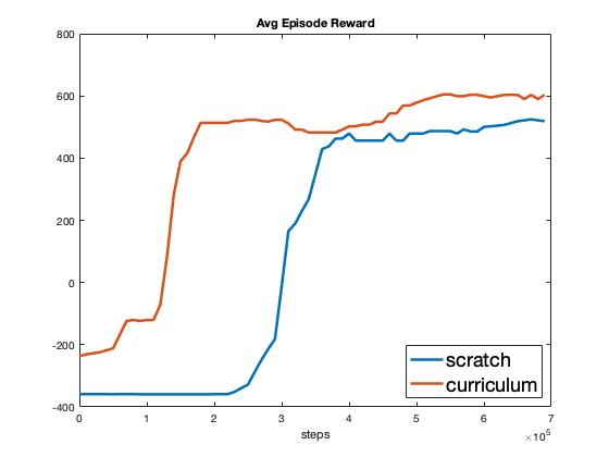
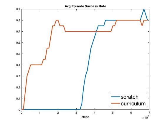
We hypothesize that the reason the scratch agent was able to match the performance of the manually designed curriculum is that there is nothing in the Stage B task that prevents the scratch agent from jointly learning Stage A from the Stage B experiences. More concretely, for the first 15 meters of the Stage B driving task, it is identical to Stage A. Only after 15 meters of driving does Stage B differ with the possibility of collision with the non-ego vehicle. Thus, Stage B is in no way structurally more difficult than Stage A, which results in the scratch agent being able to learn Stage A jointly using the first 15 meters of the task, and match the curriculum agent’s performance.
From this it was clear to us that in order to highlight the benefits of the CL, we would need to design Stage B to be structurally unique from Stage A in a fashion which would make jointly learning Stage A impossible. The only way to prevent joint learning was to design Stage B in such a way that an untrained scratch agent would not be able to gather experiences to learn Stage A while in Stage B. Thus we changed the design of Stage B to be a pedestrian crossing directly in front of the agent, which reduced the “Stage A runway" from 15 meters to <1 meter (recall the position of the pedestrian in Fig. 6). In order to learn this more difficult Stage B task, we also moved from a manually designed curriculum to the more advanced method of Automatically Generated Curriculum (AGC), discussed in the next subsection.
Automatically Generated Curriculum
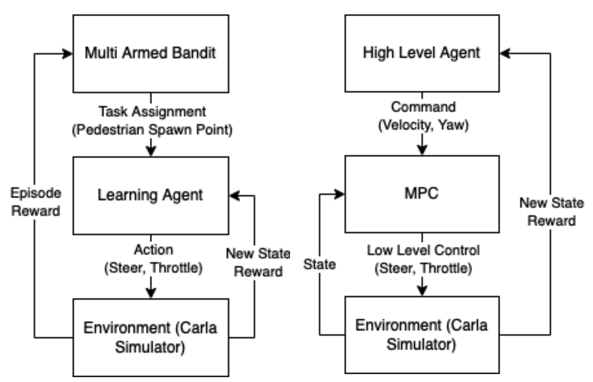
AGC for learning a difficult automated driving task set was proposed by [@qiao2018automatically], who formulated the problem of selecting which task to present the agent with next as a multi-armed bandit (illustrated in Fig. 3). In our setting, the tasks are 11 different starting positions of the crossing pedestrian: -5 meters to +5 meters laterally from the starting position of the agent. Tasks with spawn positions further from the agent are easier to learn, as a collision is inherently less likely. The proposed AGC bandit learns to assign such easy tasks to the learning agent first, moving onto the more difficult tasks afterwards. The main argument is that such a task assignment facilitates learning and leads to better learning performance compared to e.g. a random assignment of tasks.
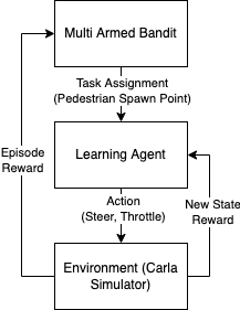
Bandit Formulation: Formally, our bandit is trying to maximize the expected cumulative reward of the learning vehicle agent it is assigning tasks to. The state space in which the bandit is operating includes both the simulator environment as well as the learning agent, however the bandit does not receive any state observations. Finally, the arms of the bandit are defined as the task set from which the bandit picks the next task assignment from. The bandit algorithm chosen was \(\epsilon\)-greedy for prototyping simplicity.
There are a couple key differences between a vanilla bandit implementation and the one proposed for AGC. First, a pruning scheme for the bandits arms is required, since we eventually want the bandit to perform well on the entire task set, and hence eventually all tasks must be assigned. We implemented pruning of task-arms based on the learning agent obtaining a >0.9 success rate on the to-be-pruned task. However, it is possible that after pruning a task, the learning agent will forget how to perform that task while learning others. Second, the fundamental bandit assumption of a static state space does not hold in the context of AGC. Since the learning agent itself is part of the state space we are extracting rewards from, and the agent is constantly changing as it learns.
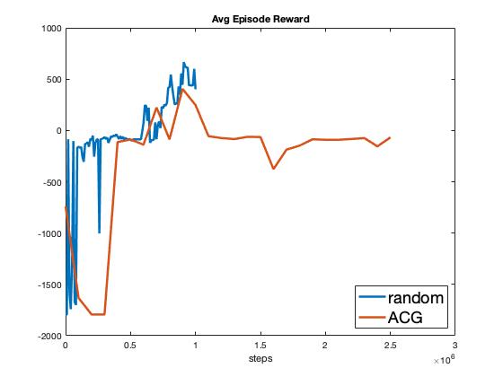
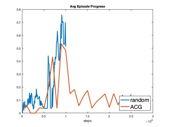
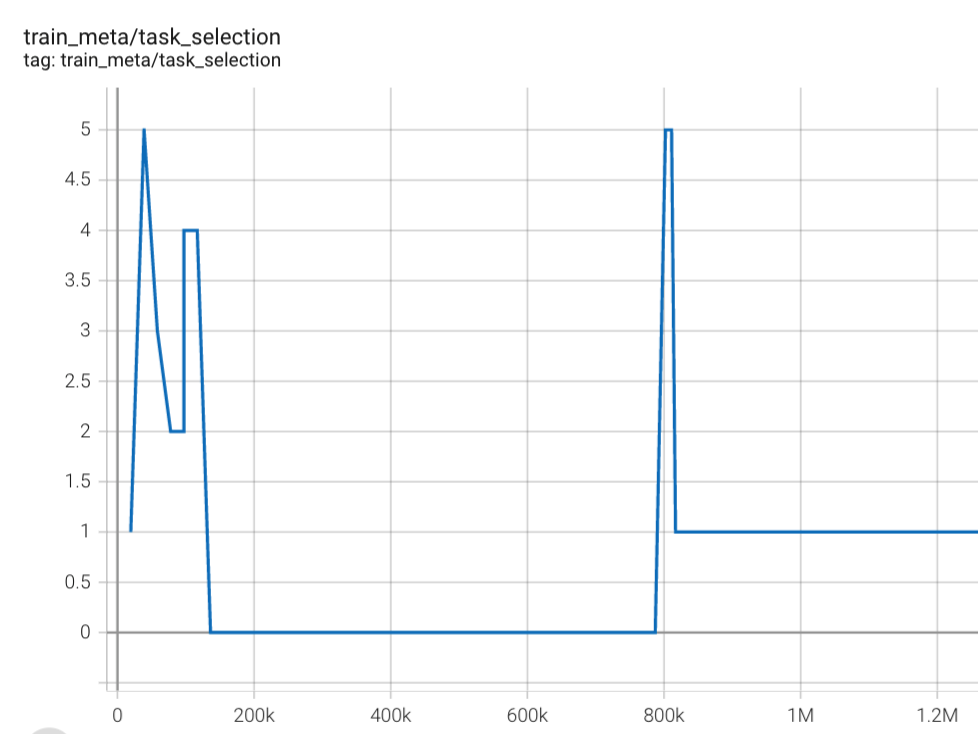
A comparison of AGC versus random task assignment over select KPIs are shown in Fig. 4. As seen in the figure, the agent learning under AGC task assignments struggles to keep up with the performance of the agent learning under random task assignment. Furthermore, after 1M experiences the performance of the AGC agent sharply drops and does not recover. The drop coincides with task 0 being pruned and task 1 starting to be assigned (see Fig. 7 in Appendix Additional Plots). From these results it is clear that the issues raised previously regarding the bandit formulation of AGC are of practical significance. Specifically, the pruning of arms does lead forgetting and drops in performance. Furthermore, the violation of the static state assumption brought on by the learning of the agent makes a bandit formulation ill-suited for AGC task assignment problem.
Algorithm Design II: Hierarchical Planning via MPC
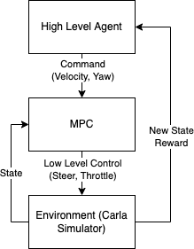
The second algorithmic modification we experimented with was introducing a hierarchical planning and control scheme, as illustrated in Fig.
- In this scheme, the learning agent’s action space is modified to be a set of high-level commands (reference velocity and yaw angle) to send to a low level Model Predictive Controller (MPC). The low level MPC then solves an optimization program online to track these reference signals.
Background and Algorithm Overview
Using hierarchical planning for mobile robotics is ubiquitous in the community, see [@7490340] for a survey and [@Daoud] for an in-depth analysis of MPC. The main idea behind using distinct high-level and low-level planners is to separate the responsibilities of the two modules, making the task that each must carry out simpler. For example, a common pattern for obstacle avoidance in mobile robotics is to have a high-level planner generate an obstacle-free trajectory, and a low-level planner then follow that trajectory. Both the generation and following tasks are separately easier tasks than the overall task of obstacle avoidance.
In our context of intersection traversal we also have an overall goal that can be broken down into easier tasks: (1) Knowing when to yield to oncoming traffic, and (2) knowing how to actuate the simulated vehicle to execute maneuvers such as lane following and yielding. Note that task (2) is very much in the wheelhouse of existing control schemes such as MPC, as it boils down to minimizing a quadratic objective defined in terms of reference errors. Task (1) on the other-hand is by no means solved in the literature, and approaches are commonly classified into two main groups: rule-based and RL-based approaches. Rule-based approaches use safety intersection metrics, e.g. time-to-intersection (TTI) and time-to-collision (TTC), to constrain the commanded actions, whereas RL approaches focus on studying the interaction between the vehicle and the intersection environment to learn an optimal crossing policy [@isele2018navigating].
Our proposal is to solve task (1) via the same formulation and RL implementations discussed in Section [2]. The only change needed is illustrated in Fig. 3: The outputs of the RL-agent are no longer interpreted as control actions imparted into the vehicle model, but rather the high level commands necessary to solve task (1). The commands are then passed onto the MPC scheme, described next, which produces the low-level control actions necessary to solve task (2).
MPC Implementation
The MPC controller tracks the lane center and the references commanded by the high level RL-agent by minimizing the objective function (Eq. (3)) and respecting the vehicle’s non-holonomic constraints by utilizing a kinematic predictive model (see Fig. 8 in Appendix MPC Implementation Details). Specifically, the objective function is a combination of: lateral deviation from the center of the lane, velocity error from reference, yaw error from reference, and the delta between control actions (to encourage smooth driving):
\[J\big(\mathbf{z},\mathbf{u}\big) = \int_{t_0}^{t_0 + T_H} \big|\big| \mathbf{z}_{ref} - \mathbf{z} \big|\big|_Q^2 + \big|\big| \mathbf{\dot{u}} \big|\big|_R^2 \tag{3}\]where \(\mathbf{z} = \begin{bmatrix} \xi & \theta & v \end{bmatrix}^\top\), \(\xi\) is the vehicle’s lateral deviation from the center of the lane, \(\theta\) is its yaw angle, and \(v\) is its velocity. Furthermore, \(Q \in \mathbb{R}^{3\times 3}\) and \(R \in \mathbb{R}^{2\times 2}\) are the tracking and input quadratic penalty matrices, \(t_0\) is the initial time, and \(T_H\) is the prediction horizon.
Finally, the MPC’s Optimal Control Problem (OCP) can be formulated as follows:
\[\begin{align} &\!\min_{\mathbf{u}(t)} &\qquad& \hspace{15mm} J(\mathbf{z}(t), \mathbf{u}(t)) \tag{4}\\ &\text{s.t.} & & \mathbf{\dot{x}}(t) = f\big(\mathbf{x}(t), \mathbf{u}(t)\big),&\hspace{0mm} \forall t \in [t_0, t_0+T_H] \tag{4a}\\ & & &\dot{\mathbf{u}}_{min}(t)\leq \dot{\mathbf{u}}(t) \leq \dot{\mathbf{u}}_{max}(t),&\forall t \in [t_0, t_0+T_H] \tag{4b}\\ & & & \mathbf{u}_{min}(t)\leq \mathbf{u}(t) \leq \mathbf{u}_{max}(t),& \forall t \in [t_0, t_0+T_H] \tag{4c} \end{align}\]\(\mathbf{\dot{x}}(t)\) is defined via the predictive model (see Appendix MPC Implementation Details), and the bounds on \(\dot{\mathbf{u}}(t), \mathbf{u}(t)\) can be found in Table [14] in Appendix MPC Implementation Details.
Results and Discussion
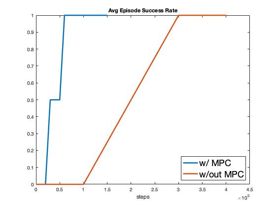
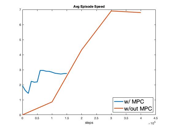
A comparison of hierarchical planning versus low-level SAC (the same agent presented in Section [2]) is shown in Fig. 5. As seen in Fig. 5, the agent operating in the hierarchical scheme learns the intersection traversal task in a fraction of the number of experiences as the low-level control model discussed in Section [2]. The reason for this is exactly what was discussed in Section [4.1]; the hierarchical agent only needs to learn task (1), which takes fewer experiences versus learning both task (1) and (2) as required of the low-level agent. Additionally, as seen in Fig. 5, the average speed of the hierarchical agent is less than half that of the low-level agent. This is not optimal from the agent’s perspective, which would like to drive at the speed limit of 12m/s, however it is optimal from a passenger comfort and safety perspective, which the input constraints specified in Eqs. (4b) and (4c) enforce.
These results present a compelling argument for not “reinventing the wheel". As RL researchers and practitioners we should think critically about where in our application’s pipeline introducing an RL agent makes the most sense. If there are parts of the application pipeline that already have strong implementations (reference tracking via MPC in our case), it is beneficial to use such implementations hand-in-hand with an RL agent, instead of replacing the entire pipeline.
Background
Additional Plots
MPC Implementation Details
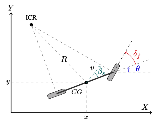
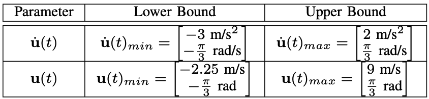
Fig. 8a illustrates the kinematic bicycle model used to predict the evolution of the vehicle’s state:
\[\mathbf{\dot{x}} (t) = \begin{bmatrix} \dot{x}\\\dot{y}\\\dot{\theta} \end{bmatrix}= f\Big(\mathbf{x}(t), \mathbf{u}(t)\Big) = \begin{bmatrix} v \cos(\theta + \beta_s)\\ v \sin(\theta + \beta_s)\\ \frac{v \cos(\beta_s) \tan(\delta_f)}{L} \end{bmatrix},\]where
\[\beta_s = \arctan \left( \frac{l_r \tan \delta_f}{L} \right)\]where the vehicle state is \(\mathbf{x} = \begin{bmatrix} x & y &\theta \end{bmatrix}^\top\), \(x\) and \(y\) are the position of the vehicle in X-Y global frame, and \(\theta\) is the vehicle orientation in the global frame. Furthermore, \(\mathbf{u} = \begin{bmatrix} v & \delta_f \end{bmatrix}^\top\) is the vector of control actions, \(v\) is the velocity of the ego vehicle at its C.G., and \(\delta_f\) is the steering angle. In Fig. 8, \(\beta_s\) is the side-slip angle of the vehicle, \(l_r\) is the distance between the rear axle and the C.G., and \(L\) is the wheelbase length of the vehicle.