COVID Outcome Prediction
Design and Implementation
To tackle the problem of COVID-19 outcome classification, three neural network architectures were applied with varying degrees of success. The architectures applied are: (1) A fully connected (FC) network, (2) a residual network (ResNet) with single layer skip-connections, and (3) a recurrent network (RNN) with long short-term memory units (LSTMs). The design and implementation details of each architecture are discussed in this section. Results and analysis are given later in section 1.3.
Fully Connected Network
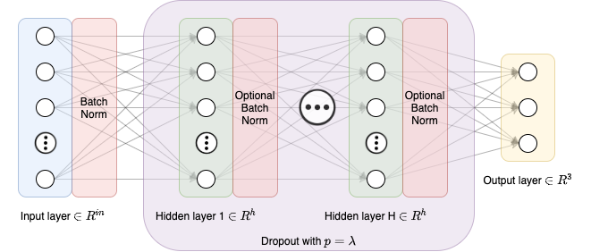 {width=”100%”}
Several different versions of FC networks were designed and implemented. These implementations varying in terms of number of input features, where batch normalization was applied, and to what degree drop-out regularization was applied. The overall architecture is captured in Fig. 1, but many different implementations are possible using the aforementioned hyperparameters. In order to categorically analyze each approach, we now define nine discrete implementations that were examined:
-
Net1: Default[^1] FC without time dimensions ($in = 49$)
-
Net2: Default FC with time dimensions ($in = 53$)
-
Net3: Default FC with time dimensions and batch norm between every hidden layer
-
Net4: Default FC with time dimensions and high drop-out ($\lambda = 0.5$)
-
Net5: Default FC with time dimensions and low drop-out ($\lambda = 0.1$)
-
Net6: Default FC with time dimensions, batch norm between every hidden layer, and high drop-out ($\lambda = 0.5$)
-
Net7: Default FC with time dimensions, batch norm between every hidden layer, and low drop-out ($\lambda = 0.1$)
-
Net8: Deep ($H=10$) FC with time dimensions and batch norm only at input
-
Net9: Deep ($H=10$) FC with time dimensions and batch norm between every hidden layer
There are also similarities across all variations implemented: The activation function used in all hidden layers is the Rectified Linear Unit (ReLU), and at the output layer is log softmax. The optimizer used for all networks is stochastic gradient descent with a batch size of 4. Negative log likelihood is used to define loss at the output layer.
Performance results and analysis of each FC network variant is given in section 1.3.
Residual Network
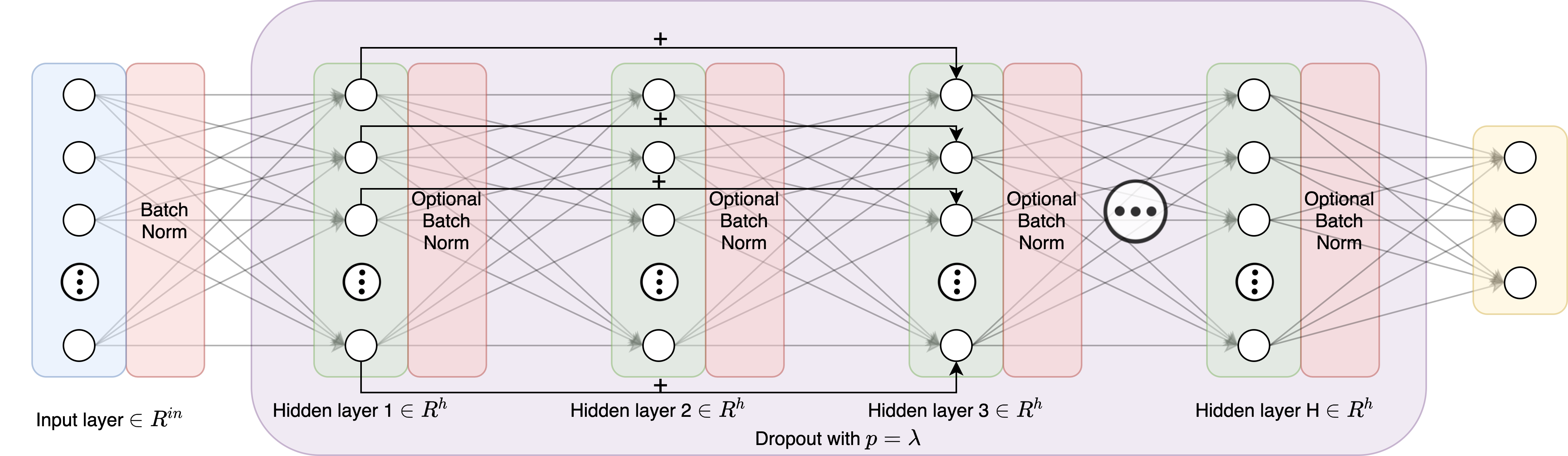 {width=”100%”}
Overall, the ResNet implementation is similar to the FC network, with the exception of the skip connections designed to allow for deeper structure without vanishing gradients. The idea here is that a deeper structure will be able to capture more complex patterns in the COVID dataset. Note that a deep structure was also implemented in the previous FC network architecture, but as discussed in section 1.3, such an implementation is likely to fall victim to the vanishing gradient problem.
The full architecture is shown in Fig. 2, which is simply an extended version of Fig. 1 with skip connections. Similar to the FC design, multiple implementations of the ResNet architecture were realized to examine the performance of different hyperparameter settings. Specifically, the implementations are as follows:
-
Net10: Shallow ResNet ($H=3$) with batch norm only at input and no drop-out
-
Net11: Deep ResNet ($H=15$) with batch norm only at input and no drop-out
-
Net12: Deep ResNet ($H=15$) with batch norm between every hidden layer and no drop-out
The activation functions, optimizer, and loss function used are the same ones used in the FC networks. Performance results and analysis of each ResNet variant are given in section 1.3.
Recurrent Network via LSTM Units
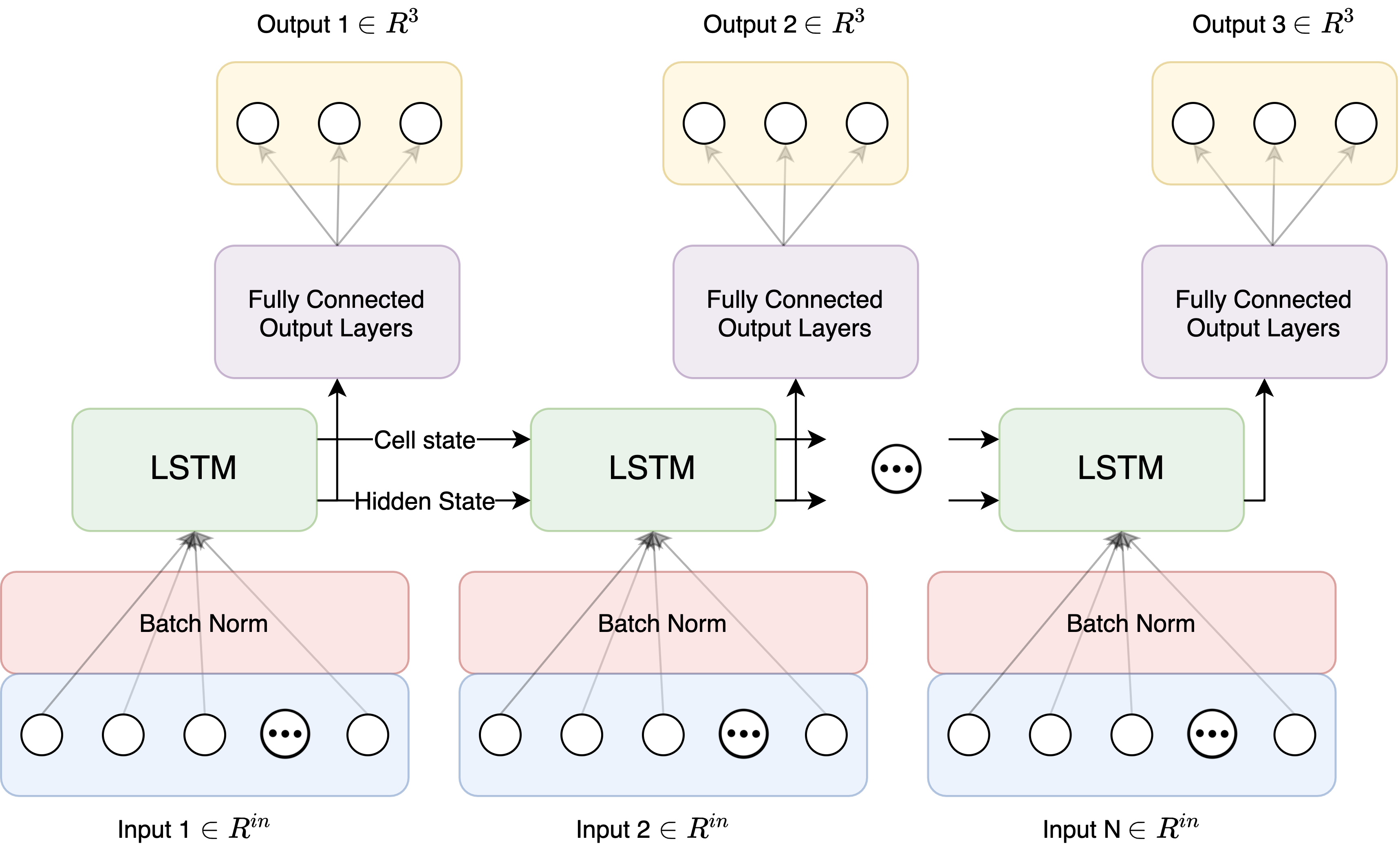 {width=”100%”}
The last network architecture that was attempted for the COVID-19 outcome classification task was a recurrent design that takes advantage of LSTM units, as shown in Fig. 3.
Network Design
The introduction of hidden state and LSTM units to the network architecture brings with it new hyperparameters to adjust. The first choice is how to map the hidden state of the network after each input instance to a classification. For this we chose a FC network, and thus any of the design parameters discussed previously in subsection 1.1.1 could be explored. However, to keep the scope of the design small, only the depth of the FC output layers was used as a hyperparameter.
Another design parameter is whether or not to stack multiple LSTM units, and if so how many. Stacking multiple LSTMs allows for greater model complexity, similar to increasing the depth in a FC network.
Dataset Design
A recurrent design also necessitates greater care of how, specifically in what order, the input instances (Input $[1…N]$) are fed into the network. If the ordering is random, we would not expect the cell state signal to carry any useful temporal information about the spreading of COVID-19 cases.
While it is clear that some ordering property much be enforced on the input sequence $[1…N]$, it is not clear at first what is the best ordering rule to maintain. For example, should the ordering be global and the cell state be maintained over all instances in the dataset; or should the dataset be broken up into multiple separate temporal sequences between which the cell state is reset, and if so how should this breaking up be done?
One way to arrive at potential answers is to think about RNNs in the context of natural language tasks such as word tagging (verb, adjective, etc...). In such tasks, input instances are usually broken up at the end of each sentence. The reasoning here is that context changes between sentences, and therefore preserving LSTM cell state over multiple sentences may cause the tagger network to be biased towards context at the end of the previous sentence, which no longer applies to the current sentence.
Motivated by NLP tasks, we can think about when context changes in our COVID-19 dataset, and a couple intuitive indicators arise: (1) COVID-19 outbreaks at different public health units (PHUs) are usually temporally independent of each other. Therefore, breaking up the dataset into temporal sequences with one sequence per PHU may allow the network to learn what the pattern of an outbreak looks like at any PHU. (2) Or, as a similar alternative, separating temporal sequences based on geographical region may yield a greater degree of independence since multiple PHUs may fall under the umbrella of the same regional outbreak. However, defining geographic regions based on the lat/lon data given is a complicated task on its own, and thus the PHU-based separation was selected for experimentation.
Implementation Variants
Given the above design concerns, several different RNN network implementations were trained to confirm or refute the hypotheses discussed above:
-
Net13: Default[^2] LSTM RNN trained with no temporal ordering on input sequence.
-
Net14: Default LSTM RNN trained with one globally ordered input sequence.
-
Net15: LSTM RNN with deep ($H=5$) output FC network and trained with one globally ordered input sequence.
-
Net16: LSTM RNN with three stacked LSTM units and trained with one globally ordered input sequence.
-
Net17: LSTM RNN with deep ($H=5$) output FC network, three stacked LSTM units, and trained with one globally ordered input sequence.
-
Net18: Default LSTM RNN trained with multiple input sequences (one per PHU), and temporally ordered within each sequence.
-
Net19: LSTM RNN with three stacked LSTM units and trained with multiple input sequences (one per PHU), and temporally ordered within each sequence.
-
Net20: LSTM RNN with five stacked LSTM units and trained with multiple input sequences (one per PHU), and temporally ordered within each sequence.
The activation functions, optimizer, and loss function used are the same ones used in the FC networks. Performance results and analysis of each LSTM RNN variant are given in section 1.3.
Implementation Details
In this section we give a high level description of the key blocks of Python and PyTorch code that implements our neural networks and conducts training and evaluation.
Fully Connected Network Implementation
class FCNet(nn.Module):
    def __init__(self, in_dimen=53, width=200, depth=3, dropout=0.0, batch_norm=False):
        self.dropout = nn.Dropout(dropout) if dropout > 0.0 else None
        self.batch_norm_every_layer = batch_norm_every_layer
        self.norm_in = nn.BatchNorm1d(in_dimen)
        self.norm_fc = nn.BatchNorm1d(width)
        while (depth > 0):
          self.fcs.append(nn.Linear(width, width))
          depth -= 1
        self.outfc = nn.Linear(width, 3)

    def forward(self, x):
        x = self.norm_in(x)
        for i, fc in enumerate(self.fcs):
          out = fc(x)
          if self.batch_norm_every_layer:
            out = self.norm_fc(out)
          x = F.relu(out)
          if self.dropout is not None and i < len(self.fcs) - 1:
            x = self.dropout(x)
        x = self.outfc(x)
        return F.log_softmax(x)
In this code we setup the necessary structure of a fully connected network in a manner that allows for easy experimentation of different implementation variants. In the constructor we allow for changes to number of input dimensions ($in_dimen$), width of the hidden layers ($width$), number of hidden layers ($depth$), dropout ratio ($dropout$), and whether or not to batch normalize in between every hidden layer or just at the input layer ($batch_norm$).
Residual Network Implementation
class ResNet(nn.Module):
    def __init__(self, in_dimen=53, width=200, depth=3, batch_norm=False):
        self.norm_in = nn.BatchNorm1d(in_dimen)
        self.norm_fc = nn.BatchNorm1d(width)
        self.batch_norm_every_layer = batch_norm_every_layer
        while (depth > 0):
          self.fcs.append(nn.Linear(width, width))
          depth -= 1
        self.outfc = nn.Linear(width, 3)

    def forward(self, x):
        x = self.norm_in(x)
        prev_x = None
        for i, fc in enumerate(self.fcs):
          out = fc(x)
          if prev_x is not None:
            out += prev_x
          if self.batch_norm_every_layer:
            out = self.norm_fc(out)
          x = F.relu(out)
          prev_x = x
        x = self.outfc(x)
        return F.log_softmax(x)
The code for the residual network architecture is the same as the FC network, allowing for the easy implementation of different variants. The only difference is the skip connection implemented in the forward step on lines 15-16.
RNN w/ LSTM Network Implementation
class GlobalLSTMNet(nn.Module):
  def __init__(self, in_dimen=53, h_dimen=64, fc_width=200, fc_depth=1, lstm_stack=1):
    self.norm_in = nn.BatchNorm1d(in_dimen)
    self.lstm = nn.LSTM(in_dimen, h_dimen, num_layers=lstm_stack)
    self.outfc = nn.Linear(hidden_dimen, 3)
    while fc_depth > 0:
      self.fcs.append(nn.Linear(fc_width, fc_width))
      fc_depth -= 1
    self.hidden_state = None
    self.cell_state = None
    self.fc_depth=fc_depth

  def forward(self, x):
    x = self.norm_in(x)
     lstm_out, (lstm_hidden, lstm_cell) =
       self.lstm(x.view(1, len(x), -1), (self.hidden_state, self.cell_state))
     for fc in self.fcs:
        tag_space = F.relu(fc(tag_space))
    tag_scores = F.log_softmax(tag_space, dim=1)
    return tag_scores

class PHULSTMNet(nn.Module):
  def __init__(self, in_dimen=53, h_dimen=64, fc_width=200, lstm_stack=1):
    self.norm_in = nn.BatchNorm1d(in_dimen)
    self.lstm = nn.LSTM(in_dimen, h_dimen, num_layers=lstm_stack)
    self.outfc = nn.Linear(hidden_dimen, 3)

  def forward(self, x):
    # x is entire input sequence for a specific PHU
    x = x[0,:,:].clone()
    xnorm = self.norm_in(x)
    lstm_out, _ = self.lstm(xnorm.view(xnorm.size()[0], 1, 53))
    tag_space = self.outfc(lstm_out.view(x.size()[0], -1))
    tag_scores = F.log_softmax(tag_space, dim=1)
    return tag_scores
There are two different implementations of the RNN architecture depending on the dataset scheme. In the global temporal dataset, the hidden state and cell state is persisted across all calls to forward because we are assuming that every data instance is from the same global instance, and therefore has shared hidden context that should be persisted. In the PHU based local temporal dataset scheme, each call to forward is an entire data sequence from one of the PHUs. Therefore we do not persist hidden state and cell state between calls to forward because the hidden context is assumed to change between PHUs.
Network Training Code
def train_net(net_to_train, train_loader, val_loader, epochs=20,
optimizer=SGD(), criterion=nn.NLLLoss()):
  for epoch in range(epochs):
    for batch_idx, (data, target) in enumerate(train_loader):
      data, target = Variable(data), Variable(target)
      optimizer.zero_grad()
      net_out = net_to_train(data)
    loss = criterion(net_out, torch.max(target, 1)[1])
    loss.backward()
    optimizer.step()
The training code is also designed to be network-agnostic, and was used to train all of the 20 variants implemented. The code uses PyTorch’s DataLoader class to easily change batch size and other implementation details such as data sequence ordering in the case of the RNN DataLoader.
Network Evaluation Code
def acc(net_to_test, test_loader, criterion):
  correct = 0
  loss = 0
  for data, target in test_loader:
      data, target = Variable(data), Variable(target)
      net_out = net_to_test(data)
      pred = net_out.data.max(1)[1]
      loss += criterion(net_out, torch.max(target, 1)[1])
      correct += pred.eq(torch.max(target, 1)[1]).sum().detach()
  return (loss / total, correct / total)
Unlike the previous training code, this accuracy evaluation method takes the validation dataset DataLoaders and computes loss and accuracy metrics based on that validation dataset.
Results Analysis
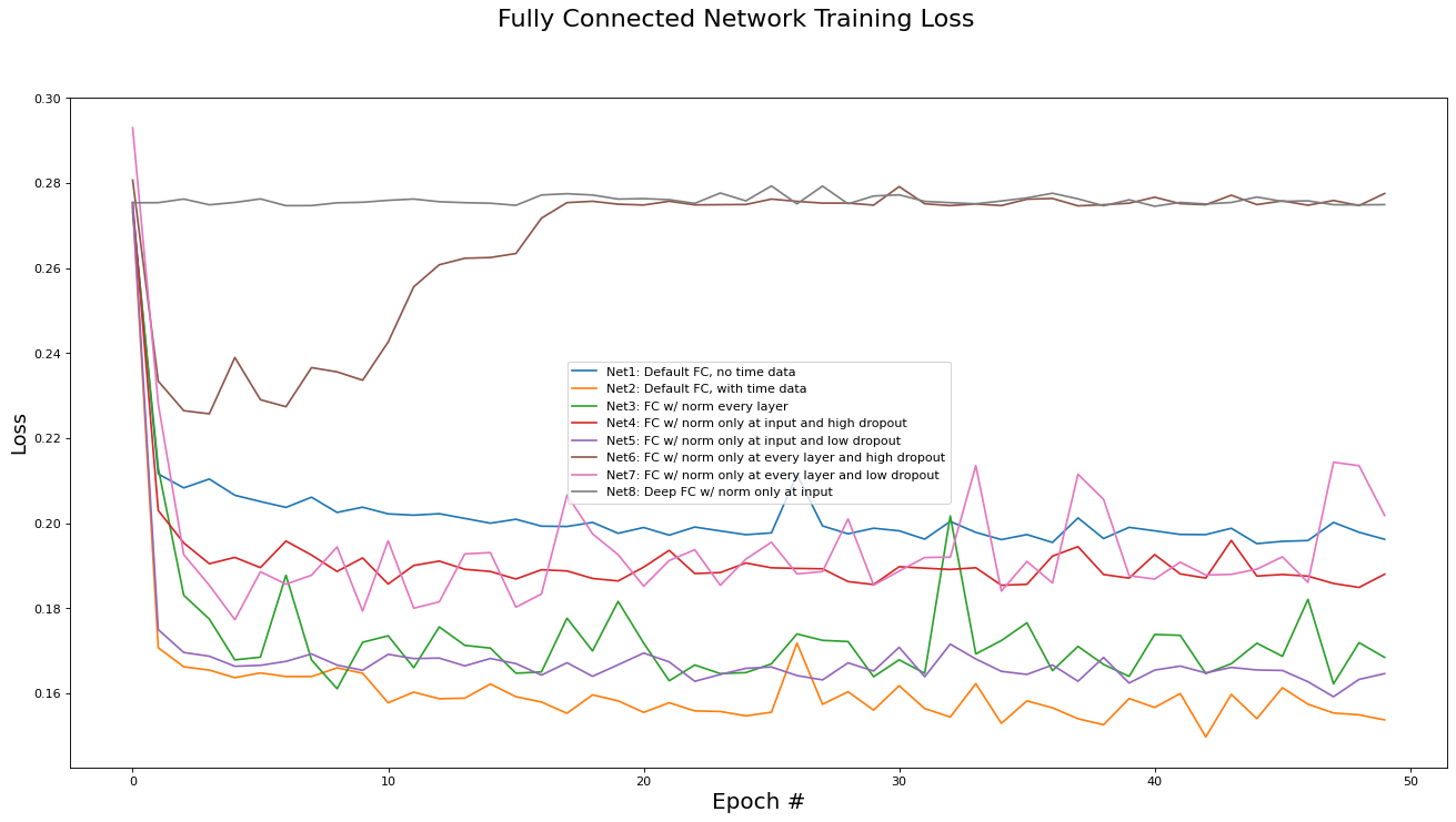
Fully Connected Network Results Analysis
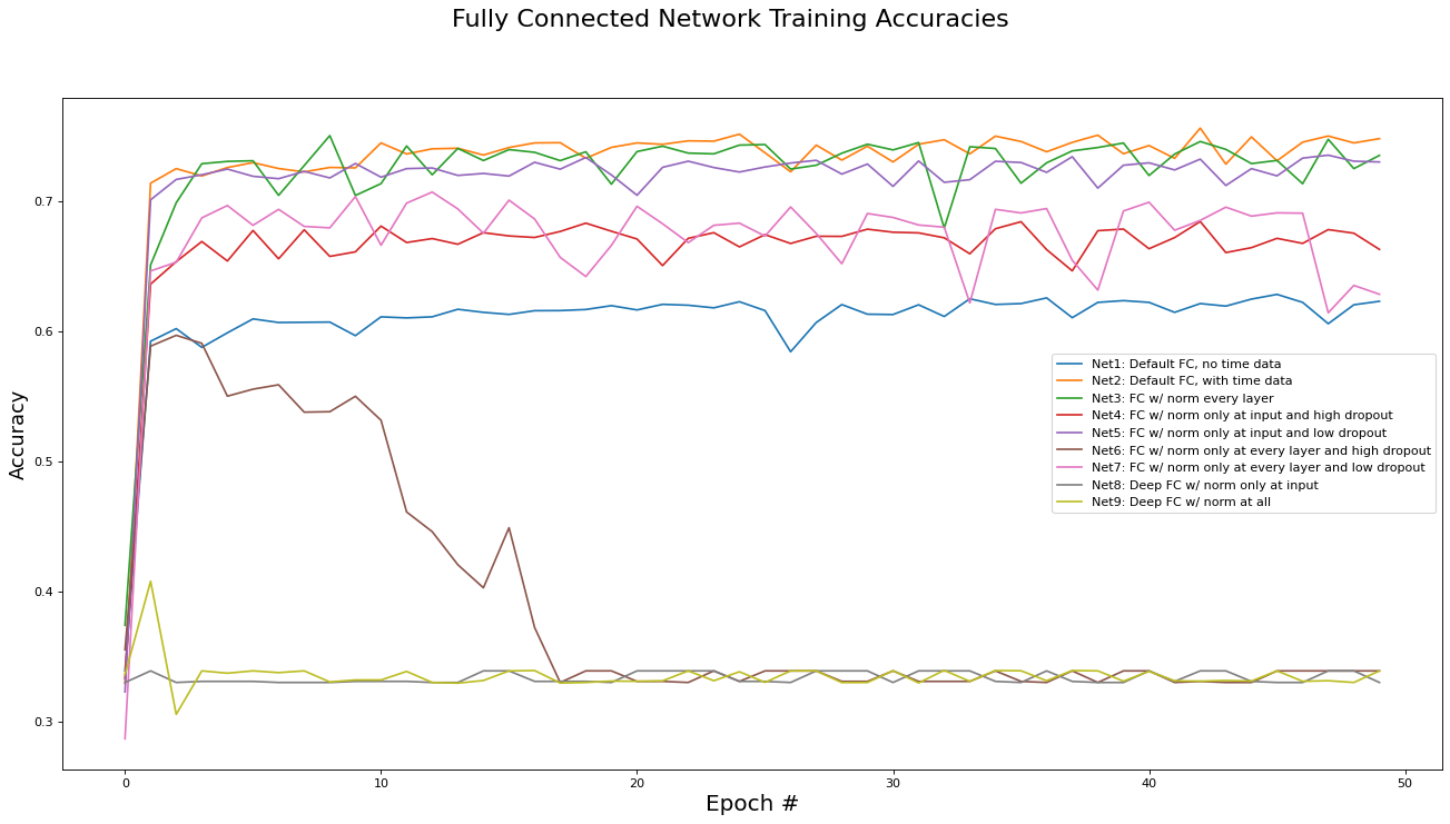
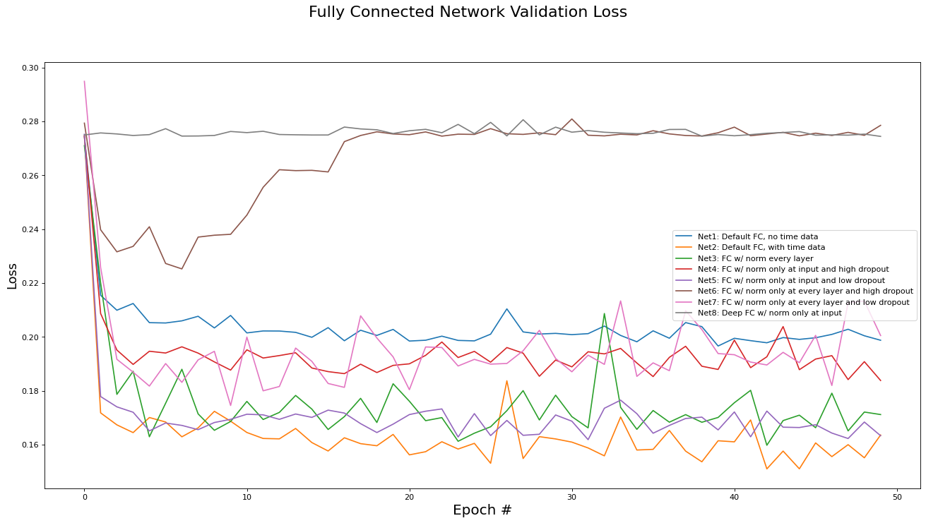
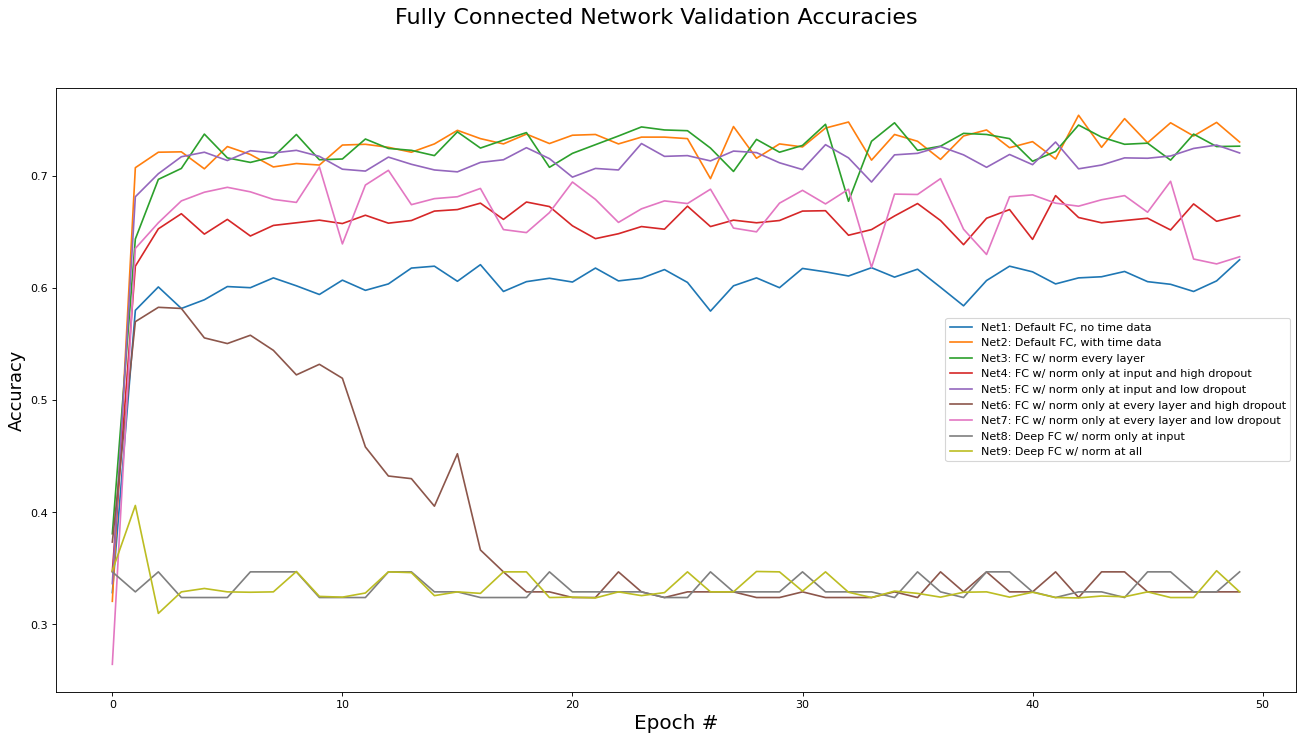
This subsection analyzes the performance of the fully connected networks (Net[0...9]). The metrics analyzed are training set loss, training set accuracy, validation set loss, and validation set accuracy. Results are presented in the epoch graphs of Fig 4. below:
::: {.figure*}
 {#fig:mean and std of net14
width=”\textwidth”}
{#fig:mean and std of net14
width=”\textwidth”}
 {#fig:mean and std of net24
width=”\textwidth”}
{#fig:mean and std of net24
width=”\textwidth”}
 {#fig:mean and std of net34
width=”\textwidth”}
{#fig:mean and std of net34
width=”\textwidth”}
 {#fig:mean and std of net44
width=”\textwidth”}
:::
{#fig:mean and std of net44
width=”\textwidth”}
:::
As seen in Fig. 4, the best parameter setting for the fully connected network is:
-
Best Fully Connected network for Training Loss is ‘Net2: Default FC, with time data’ with metric of 0.1497 at epoch# 42
-
Best Fully Connected network for Training Accs is ‘Net2: Default FC, with time data’ with metric of 0.7561 at epoch# 42
-
Best Fully Connected network for Validate Loss is ‘Net2: Default FC, with time data’ with metric of 0.1510 at epoch# 42
-
Best Fully Connected network for Validate Accs is ‘Net2: Default FC, with time data’ with metric of 0.7540 at epoch# 42
Training runtime and inference runtime data was also collected and is reported here:
-
Net1: Average training runtime: 6 seconds per epoch. Average test inference runtime: 0.4 milliseconds per instance.
-
Net2: Average training runtime: 6 seconds per epoch. Average test inference runtime: 0.4 milliseconds per instance.
-
Net3: Average training runtime: 24 seconds per epoch. Average test inference runtime: 2.0 milliseconds per instance.
-
Net4: Average training runtime: 6 seconds per epoch. Average test inference runtime: 0.5 milliseconds per instance.
-
Net5: Average training runtime: 6 seconds per epoch. Average test inference runtime: 0.5 milliseconds per instance.
-
Net6: Average training runtime: 25 seconds per epoch. Average test inference runtime: 2.2 milliseconds per instance.
-
Net7: Average training runtime: 25 seconds per epoch. Average test inference runtime: 2.2 milliseconds per instance.
-
Net8: Average training runtime: 9.8 seconds per epoch. Average test inference runtime: 0.75 milliseconds per instance.
-
Net9: Average training runtime: 70 seconds per epoch. Average test inference runtime: 6.5 milliseconds per instance.
The results presented above also tell us about the efficacy of the parameters used in the other implementation variants:
-
The instance time dimensions were crucial for performance. Net2 (with time data) outperformed Net1 (without time data) by 10%. This is motivation that a RNN may be able to achieve even better results by taking advantage of the structure inherent in the temporal dimensions.
-
Batch norming between every hidden layer (Net3) versus only at the input layer (Net2) did not yield any difference in performance. Thus, since batch norming at each layer increases training time by a factor of 4, batch norming at only the input layer is preferred.
-
Applying drop-out regularization decreased training accuracy, as expected, however it also decreased validation accuracy instead of increasing it. We conclude that dropout regularization is not needed for the COVID-19 dataset as there is minimal overfitting without any regularization methods (see validation accuracy plot versus training accuracy plot). This may be because the large volume of data acts as a regularizer on its own.
-
The deep variants (Net8 and Net9) did not appear to be trained at all. This is most likely due to the vanishing gradient problem, which will be addressed via ResNets in the next subsection.
Residual Network Results Analysis
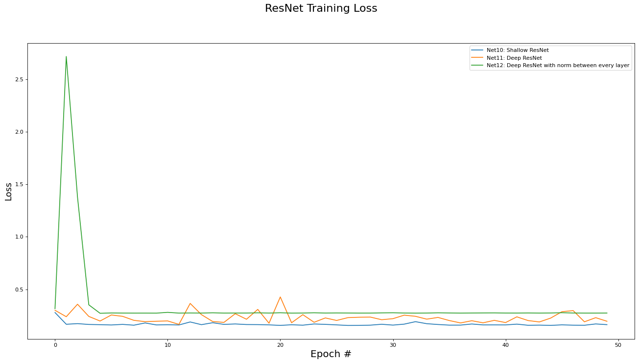
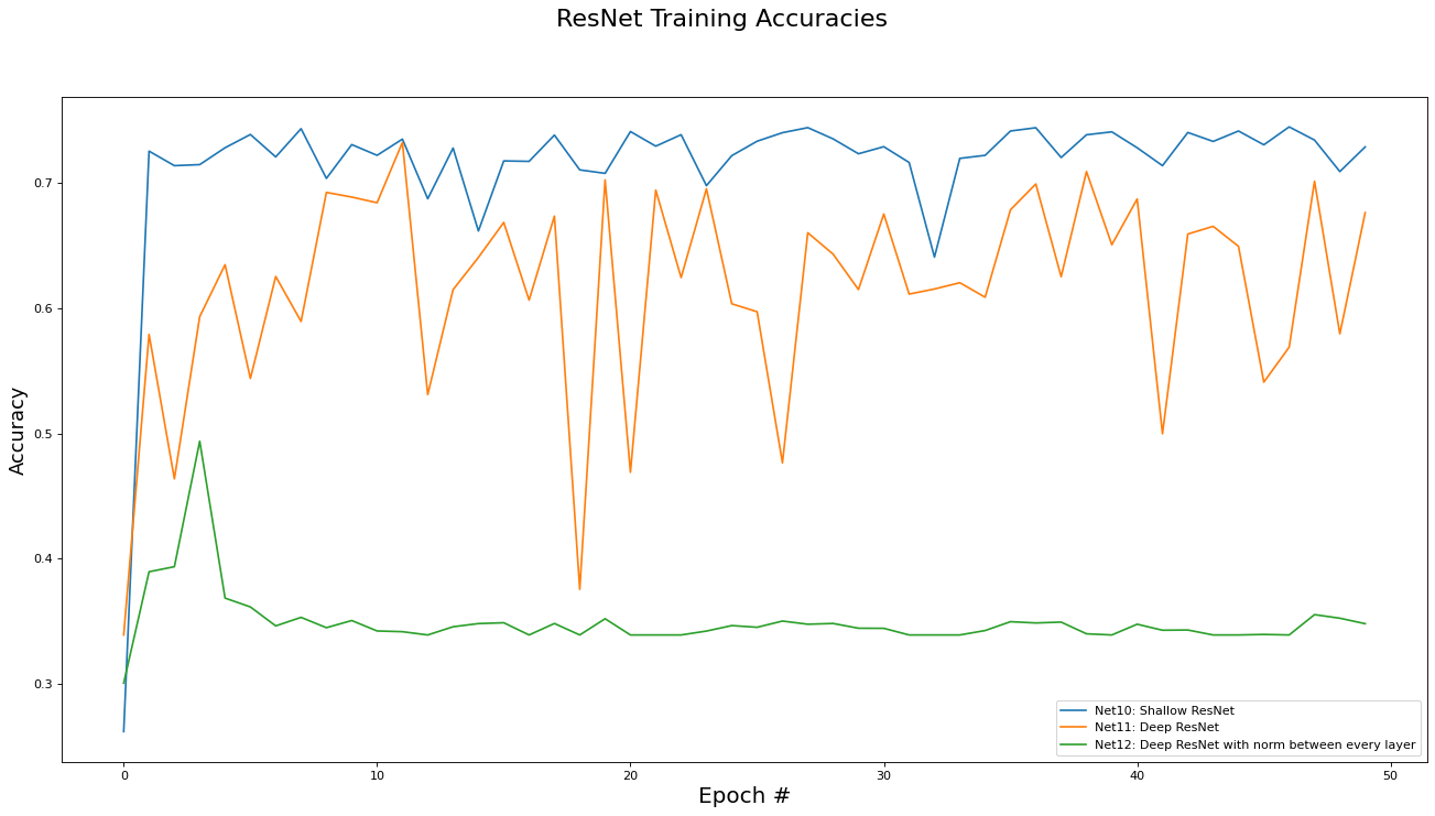
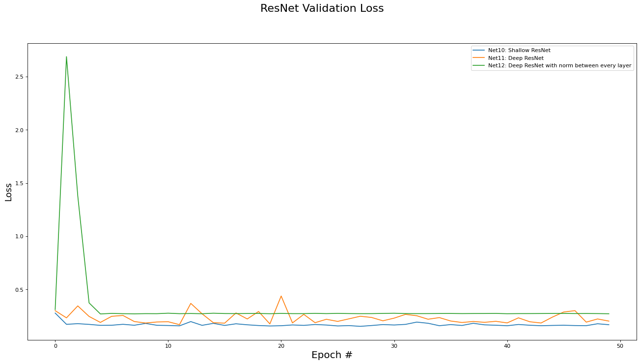
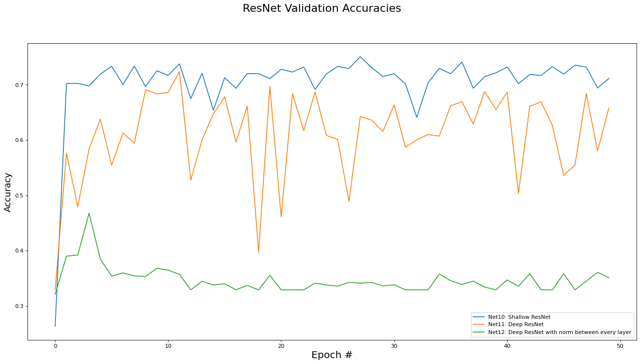
This subsection analyzes the performance of the Residual networks (Net[10,11,12]). The metrics analyzed are training set loss, training set accuracy, validation set loss, and validation set accuracy. Results are presented in the epoch graphs of Fig 5. below:
::: {.figure*}
 {#fig:mean and std of net14
width=”\textwidth”}
{#fig:mean and std of net14
width=”\textwidth”}
 {#fig:mean and std of net24
width=”\textwidth”}
{#fig:mean and std of net24
width=”\textwidth”}
 {#fig:mean and std of net34
width=”\textwidth”}
{#fig:mean and std of net34
width=”\textwidth”}
 {#fig:mean and std of net44
width=”\textwidth”}
:::
{#fig:mean and std of net44
width=”\textwidth”}
:::
As seen in Fig. 5, the best parameter setting for the Residual network is:
-
Best Residual network for Training Loss is ‘Net10: Shallow ResNet’ with metric of 0.1559 at epoch# 26
-
Best Residual network for Training Accs is ‘Net10: Shallow ResNet’ with metric of 0.7447 at epoch# 46
-
Best Residual network for Validate Loss is ‘Net10: Shallow ResNet’ with metric of 0.1543 at epoch# 27
-
Best Residual network for Validate Accs is ‘Net10: Shallow ResNet’ with metric of 0.7506 at epoch# 27
Training runtime and inference runtime data was also collected and is reported here:
-
Net10: Average training runtime: 6 seconds per epoch. Average test inference runtime: 0.43 milliseconds per instance.
-
Net11: Average training runtime: 14 seconds per epoch. Average test inference runtime: 1.0 milliseconds per instance.
-
Net12: Average training runtime: 103 seconds per epoch. Average test inference runtime: 9.6 milliseconds per instance.
Comparing these ResNet results to the FC network results, we see that introducing the skip connections in the ResNet architecture did enable to the deeper variants of the networks (e.g. Net11) to be trained (i.e. somewhat obviated the vanishing gradient problem). However, the deeper residual architecture failed to out perform the shallower ones (e.g Net 2 and Net10 versus Net11), which may mean that the inherent complexity of the dataset is low enough for a shallow, small capacity, network to capture.
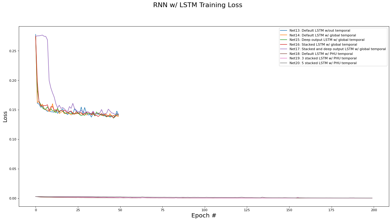
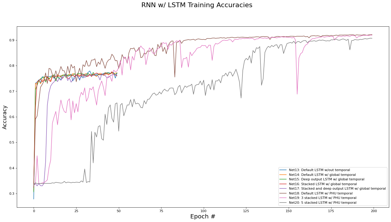
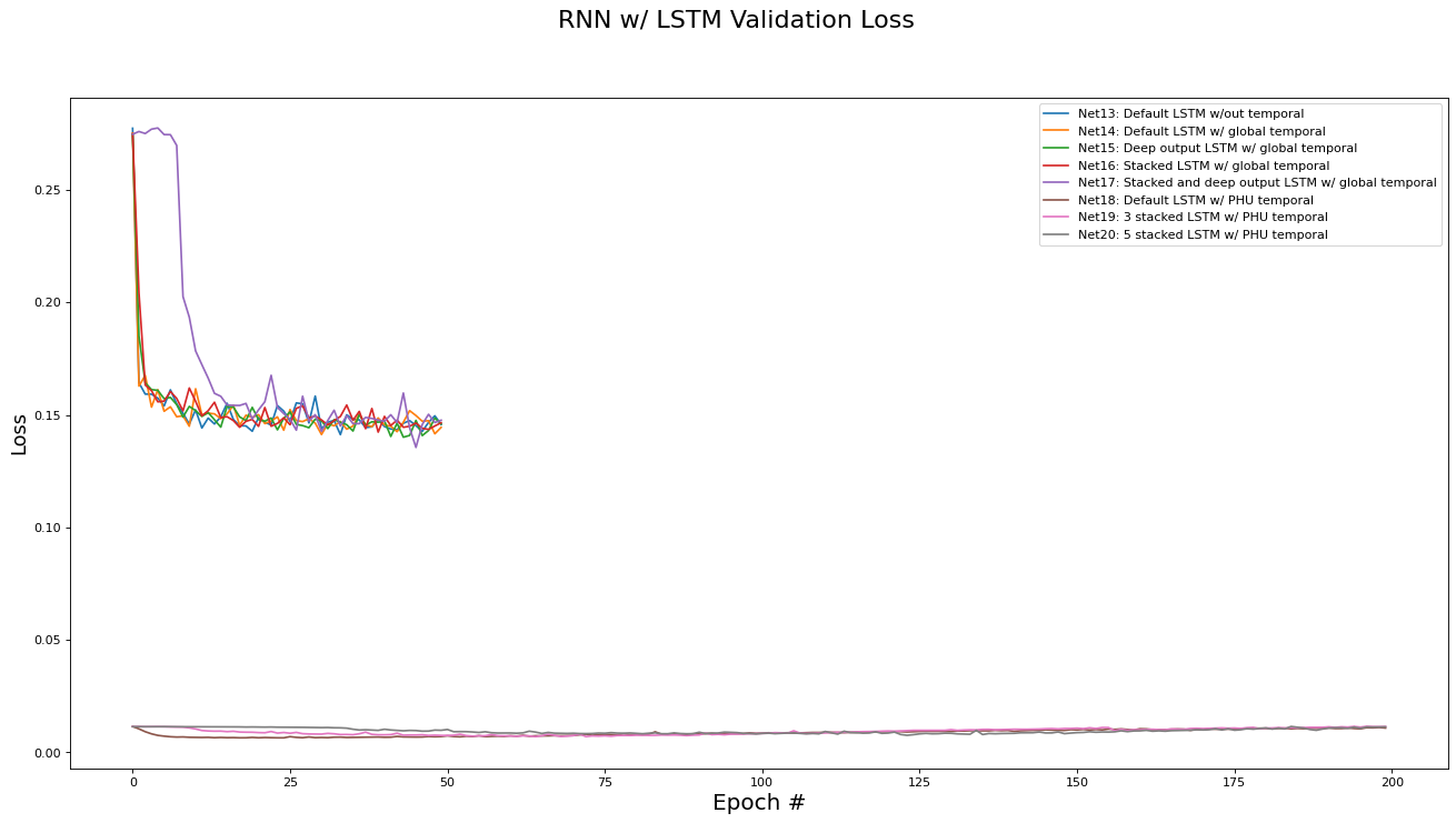
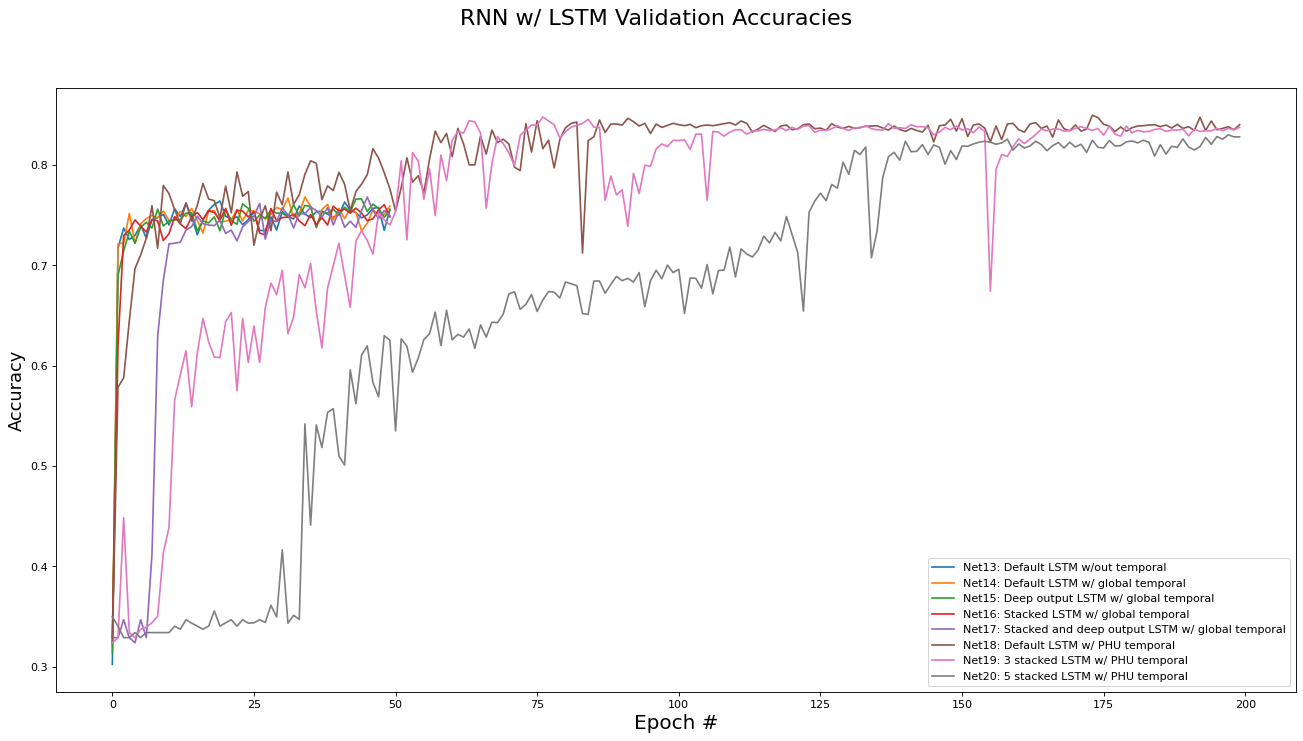
RNN via LSTM Results Analysis
This subsection analyzes the performance of the RNN/LSTM networks (Net[13...20]). The metrics analyzed are training set loss, training set accuracy, validation set loss, and validation set accuracy. Results are presented in the epoch graphs of Fig 6. below:
::: {.figure*}
 {#fig:mean and std of net14
width=”\textwidth”}
{#fig:mean and std of net14
width=”\textwidth”}
 {#fig:mean and std of net24
width=”\textwidth”}
{#fig:mean and std of net24
width=”\textwidth”}
 {#fig:mean and std of net34
width=”\textwidth”}
{#fig:mean and std of net34
width=”\textwidth”}
 {#fig:mean and std of net44
width=”\textwidth”}
:::
{#fig:mean and std of net44
width=”\textwidth”}
:::
As seen in Fig. 6, the best parameter setting for the RNN/LSTM network architecture is:
-
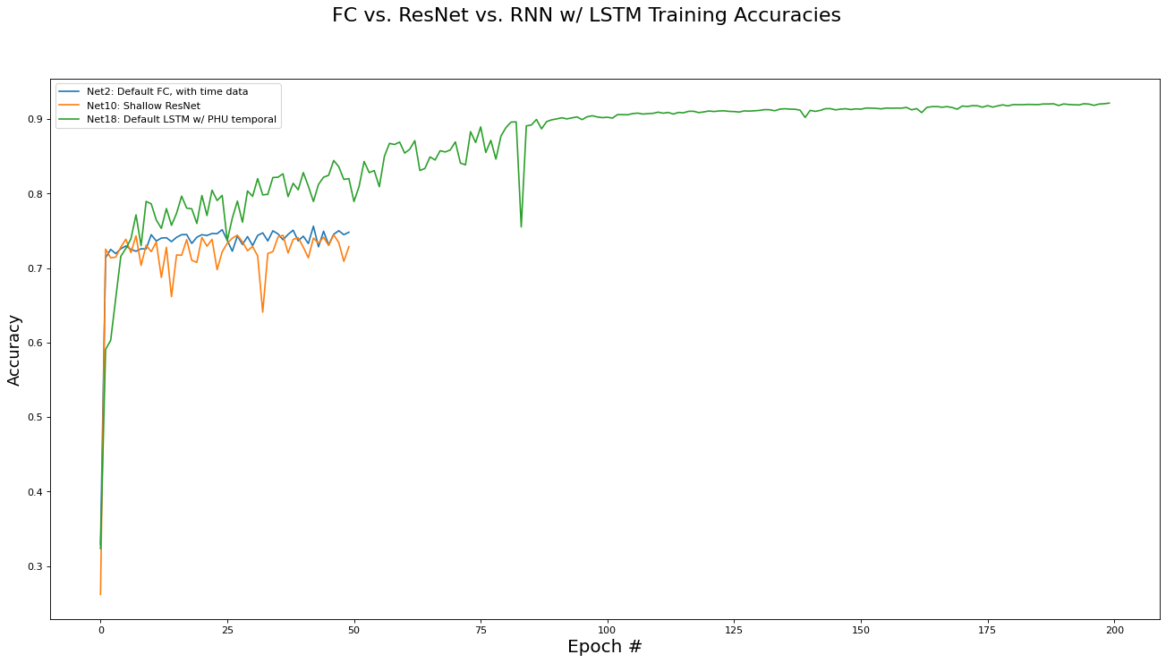
Best RNN network for Training Loss is ‘Net18: Default LSTM w/ PHU temporal’ with metric of 0.0003 at epoch# 199
-
Best RNN network for Training Accs is ‘Net18: Default LSTM w/ PHU temporal’ with metric of 0.9214 at epoch# 199
-
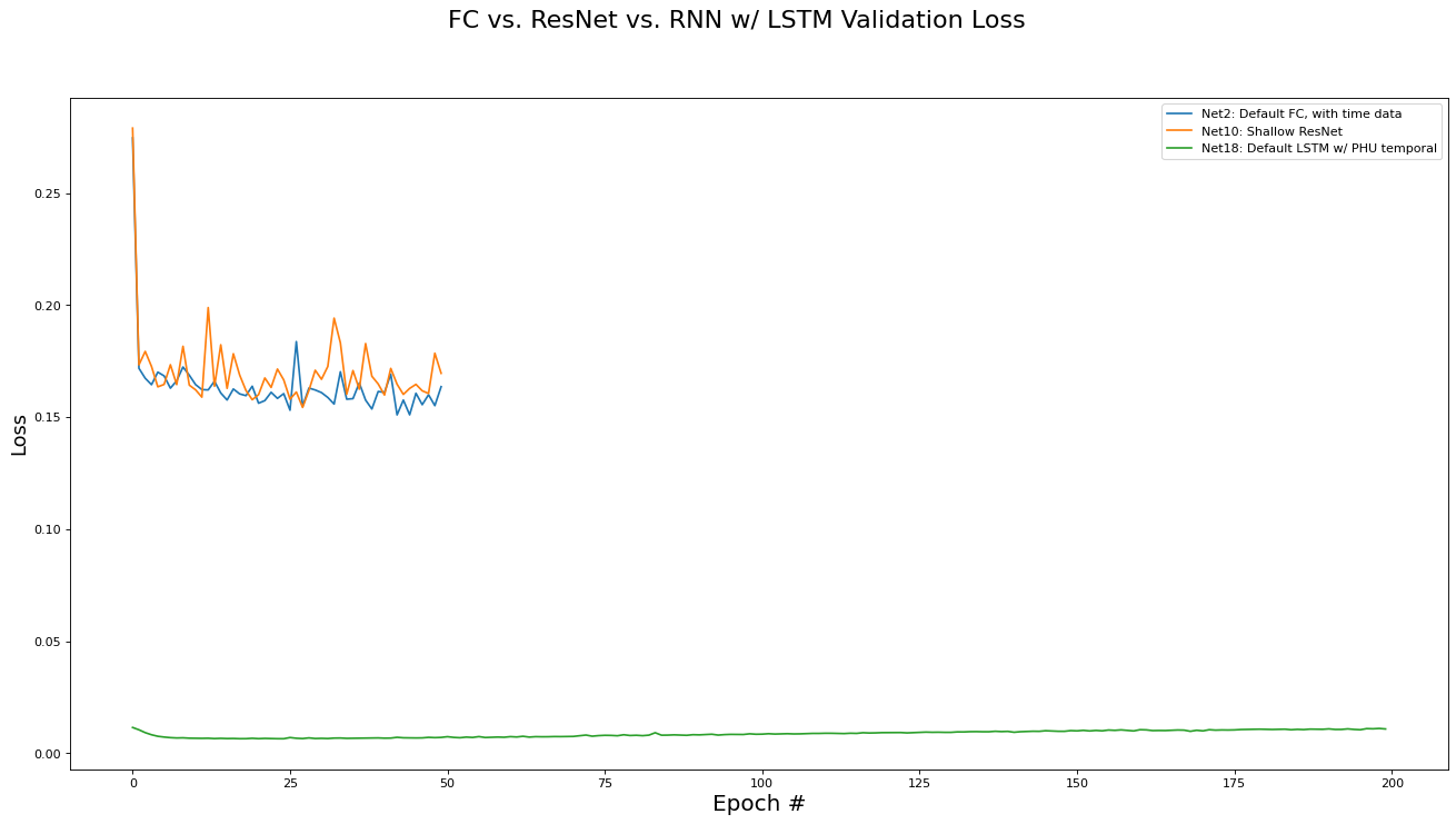
Best RNN network for Validate Loss is ‘Net18: Default LSTM w/ PHU temporal’ with metric of 0.0064 at epoch# 24
-
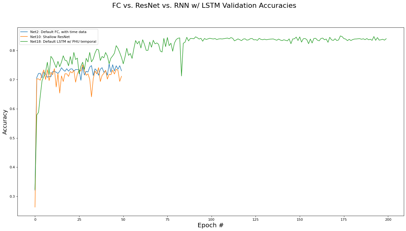
Best RNN network for Validate Accs is ‘Net18: Default LSTM w/ PHU temporal’ with metric of 0.8500 at epoch# 173
Training runtime and inference runtime data was also collected and is reported here:
-
Net13: Average training runtime: 6.7 seconds per epoch. Average test inference runtime: 0.48 milliseconds per instance.
-
Net14: Average training runtime: 6.6 seconds per epoch. Average test inference runtime: 0.48 milliseconds per instance.
-
Net15: Average training runtime: 8 seconds per epoch. Average test inference runtime: 0.7 milliseconds per instance.
-
Net16: Average training runtime: 10 seconds per epoch. Average test inference runtime: 0.7 milliseconds per instance.
-
Net17: Average training runtime: 12.5 seconds per epoch. Average test inference runtime: 0.9 milliseconds per instance.
-
Net18: Average training runtime: 3.2 seconds per epoch. Average test inference runtime: 25 milliseconds per instance.
-
Net19: Average training runtime: 8.8 seconds per epoch. Average test inference runtime: 70 milliseconds per instance.
-
Net20: Average training runtime: 15 seconds per epoch. Average test inference runtime: 112 milliseconds per instance.
There are a few interesting trends in the the RNN/LSTM variants’ performance:
-
Overall, using a recurrent architecture did improve the performance of the classifier, although by how much depending largely on which variant was used.
-
Surprisingly, enforcing a global temporal ordering at training time did not yield a performance improvement over a random ordering, but both variants did show a modest validation accuracy improvement of 2-3% over the fully connected and residual architectures.
The similar performance between the random and global ordering variants can be explained by thinking about the context of two sequential instances in the global ordering: It is unlikely that the two instances, which are likely to occur in different regions of Ontario, have any shared context. Therefore, it is actually not surprising that there is no performance difference in the two variants, since global ordering is equivalent to random ordering from the perspective of shared context. -
As hypothesized in section 1.1, crafting a dataset with local temporal ordering on a per-PHU basis lead to a large increase in performance (10% over all other methods). However, it took longer for the network to converge to this performance, needing 200 epochs to reach convergence, with a total training time of 10 minutes for the unstacked version and 50 minutes for the 5-stacked version.
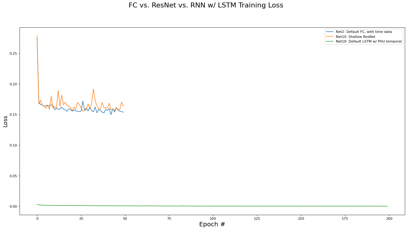
FC versus ResNet versus RNN Comparison Analysis
We conclude with a comparison of the three different network architectures discussed in this paper: Fully Connected, Residual, and RNN/LSTM networks. Note that the best performing implementation variant for each architecture category are used for comparison. The metrics analyzed are training set loss, training set accuracy, validation set loss, and validation set accuracy. Results are presented in the epoch graphs of Fig 7. below:
::: {.figure*}
 {#fig:mean and std of net14
width=”\textwidth”}
{#fig:mean and std of net14
width=”\textwidth”}
 {#fig:mean and std of net24
width=”\textwidth”}
{#fig:mean and std of net24
width=”\textwidth”}
 {#fig:mean and std of net34
width=”\textwidth”}
{#fig:mean and std of net34
width=”\textwidth”}
 {#fig:mean and std of net44
width=”\textwidth”}
:::
{#fig:mean and std of net44
width=”\textwidth”}
:::
As seen in Fig. 7, the LSTM based network in the per-PHU temporal setting largely outperforms the non-recurrent architectures, achiever 85% accuracy on the validation set.